A normal Queue follows FIFO — First In, First Out. Elements are inserted from the rear and removed from the front.
But a normal array-based Queue has an interesting problem.
Imagine a queue with five positions:
Index:    0    1    2    3    4
         [10] [20] [30] [40] [50]
          ↑                   ↑
        Front                Rear
The queue is full.
Now suppose we dequeue three elements:
Index:    0      1      2    3    4
         [  ]   [  ]   [  ] [40] [50]
                             ↑    ↑
                          Front  Rear
There are now three empty positions at the beginning. But in a simple linear queue, rear has already reached the end of the array, so those positions may not be reused.
This is where the Circular Queue comes in.
What is a Circular Queue?
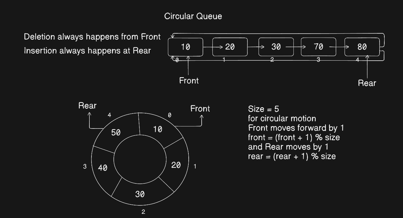
A Circular Queue is a Queue in which the last position of the underlying array is connected back to the first position.
Conceptually:
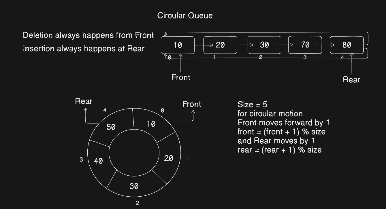
When rear reaches the last index, it can wrap around to index 0 if space is available.
This makes better use of the fixed-size array.
A Circular Queue still follows:
FIFO — First In, First Out
The difference is in how we manage the available positions.
Front and Rear
A Circular Queue normally maintains two variables:
front— points to the element that will be removed next.rear— points to the position where the latest element was inserted.
For an empty queue:
front = -1
rear = -1
For example, after inserting the first element:
Index:    0    1    2    3    4
         [10] [ ]  [ ]  [ ]  [ ]
          ↑
       front/rear
Now:
front = 0
rear = 0
After inserting more elements:
Index:    0    1    2    3    4
         [10] [20] [30] [40] [ ]
          ↑                   ↑
        Front                Rear
So:
front = 0
rear = 3
Why Do We Need %?
The most important part of a Circular Queue is the modulo (%) operator.
Suppose the queue size is 5.
The valid indexes are:
0 1 2 3 4
What happens when rear is at index 4 and we want to move it forward?
Normally:
4 + 1 = 5
But index 5 doesn't exist. (we are talking about fixed size memory)
Using modulo:
(4 + 1) % 5
= 5 % 5
= 0
So rear wraps back to index 0.
This gives us the fundamental circular movement formula:
(rear + 1) % size
The same idea is used when moving front:
(front + 1) % size
Conditions of a Circular Queue
Before implementing a Circular Queue, we need to understand its important conditions.
1. Empty Queue
The queue is empty when:
front = -1
We also maintain:
rear = -1
So the initial state is:
front = rear = -1
2. First Element Insertion
When the first element is inserted:
front = rear = 0
The first element is placed at index 0.
3. Queue is Full
A Circular Queue is full when the next position of rear is front.
The condition is:
(rear + 1) % size == front
For example, with a queue of size 5:
Index:    0    1    2    3    4
         [10] [20] [30] [40] [50]
          ↑                   ↑
        Front                Rear
Here:
(rear + 1) % size
= (4 + 1) % 5
= 0
And:
front = 0
Therefore:
(rear + 1) % size == front
The queue is full.
This is the overflow condition.
4. Deleting an Element
When deleting an element, we remove the element at front.
Then front moves forward:
front = (front + 1) % size
If the deleted element was the last remaining element, we reset:
front = rear = -1
This brings the queue back to its initial empty state.
Circular Queue Operations
A Circular Queue mainly supports:
Enqueue
Insert an element at the rear.
enqueue → rear moves
rear = (rear + 1) % size
Dequeue
Remove an element from the front.
dequeue → front moves
front = (front + 1) % size
isEmpty
Checks whether:
front == -1
isFull
Checks whether:
(rear + 1) % size == front
Circular Queue Implementation in Python
Unlike some of my earlier Queue and Deque implementations, this time I am not using Python's built-in append(), pop(), insert(), or deque operations to implement the core behavior.
Instead, this implementation uses a fixed-size list and manually manages:
frontrearoverflow
underflow
circular movement
This is much closer to the traditional array-based implementation that can be translated to languages such as C, C++, or Java.
class CircularQueue:
    def __init__(self, size):
        self.size = size
        self.items = [None] * size
        self.front = self.rear = -1

    def isEmpty(self):
        return self.front == -1

    def isFull(self):
        return (self.rear + 1) % self.size == self.front

    def enqueue(self, value):
        if self.isFull():
            print(value, "Can't be inserted, the Circular Queue is full")

        elif self.isEmpty():
            self.front = self.rear = 0
            self.items[self.rear] = value
            print("The first element has been inserted:", value)

        else:
            self.rear = (self.rear + 1) % self.size
            self.items[self.rear] = value
            print("Element inserted:", value)

    def dequeue(self):
        if self.isEmpty():
            print("The Circular Queue is empty")

        elif self.front == self.rear:
            print(self.items[self.front], "the last element has been dequeued")

            self.items[self.front] = None
            self.front = self.rear = -1

        else:
            print(self.items[self.front], "has been dequeued")

            self.items[self.front] = None
            self.front = (self.front + 1) % self.size

    def printCQ(self):
        print("The current status of the queue is:", self.items)
Understanding Enqueue
Let's look at the most important part:
self.rear = (self.rear + 1) % self.size
Suppose:
size = 5
rear = 4
Then:
rear = (4 + 1) % 5
rear = 0
So the rear wraps around.
For example:
Before:

Index:    0      1      2    3    4
         [None] [None] [None][40] [50]
                              ↑     ↑
                            Front  Rear
Now insert 60.
The new rear becomes:
(4 + 1) % 5 = 0
So:
Index:    0    1      2      3    4
         [60] [None] [None] [40][50]
          ↑                       ↑
         Rear                    Front
The physical array looks unusual, but the logical Circular Queue is:
40 → 50 → 60
This is the key idea behind a Circular Queue.
Understanding Dequeue
For deletion:
self.items[self.front] = None
self.front = (self.front + 1) % self.size
The first statement clears the old position.
The second moves front to the next position.
For example:
Before:

[10] [20] [30] [40] [50]
 ↑
front
After dequeue:
[None] [20] [30] [40] [50]
         ↑
       front
The queue now starts from 20.
The Last Element Case
There is a special condition:
self.front == self.rear
This means that the queue currently contains one element, assuming the queue is not empty.
For example:
Index:    0    1    2    3    4
         [ ]  [ ]  [ ] [40] [ ]
                       ↑
                  front/rear
Since both front and rear point to the same position, deleting this element means the queue becomes empty.
Therefore:
self.front = self.rear = -1
We also clear the array position:
self.items[self.front] = None
before resetting the indices.
Testing the Circular Queue
Let's create a Circular Queue of size 5:
cq = CircularQueue(5)
Initially:
front = -1
rear = -1
Trying to dequeue:
cq.dequeue()
produces:
The Circular Queue is empty
Now insert five elements:
cq.enqueue(10)
cq.enqueue(20)
cq.enqueue(30)
cq.enqueue(40)
cq.enqueue(50)
The array becomes:
[10, 20, 30, 40, 50]
Now try inserting another element:
cq.enqueue(60)
The Circular Queue is full, so:
60 Can't be inserted, the Circular Queue is full
This is an overflow condition.
Reusing Empty Positions
Now remove three elements:
cq.dequeue()
cq.dequeue()
cq.dequeue()
The array becomes:
[None, None, None, 40, 50]
Now there are three available positions at the beginning.
Insert 60:
cq.enqueue(60)
Since rear wraps around:
(4 + 1) % 5 = 0
the value 60 is inserted at index 0.
The array becomes:
[60, None, None, 40, 50]
The logical queue is:
40 → 50 → 60
This is the major advantage of a Circular Queue.
Complete Example
class CircularQueue:
    def __init__(self, size):
        self.size = size
        self.items = [None] * size
        self.front = self.rear = -1

    def isEmpty(self):
        return self.front == -1

    def isFull(self):
        return (self.rear + 1) % self.size == self.front

    def enqueue(self, value):
        if self.isFull():
            print(value, "can't be inserted, the Circular Queue is full")

        elif self.isEmpty():
            self.front = self.rear = 0
            self.items[self.rear] = value
            print("The first element has been inserted:", value)

        else:
            self.rear = (self.rear + 1) % self.size
            self.items[self.rear] = value
            print("Element inserted:", value)

    def dequeue(self):
        if self.isEmpty():
            print("The Circular Queue is empty")

        elif self.front == self.rear:
            print(self.items[self.front], "the last element has been dequeued")
            self.items[self.front] = None
            self.front = self.rear = -1

        else:
            print(self.items[self.front], "has been dequeued")
            self.items[self.front] = None
            self.front = (self.front + 1) % self.size

    def printCQ(self):
        print("The current status of the queue is:", self.items)


cq = CircularQueue(5)

cq.dequeue()

cq.enqueue(10)
cq.enqueue(20)
cq.enqueue(30)
cq.enqueue(40)
cq.enqueue(50)
cq.enqueue(60)

cq.printCQ()

cq.dequeue()
cq.dequeue()
cq.dequeue()

cq.printCQ()

cq.enqueue(60)

cq.printCQ()

cq.dequeue()
cq.dequeue()
cq.dequeue()
cq.dequeue()
The important states are:
Initial:
[None, None, None, None, None]

After five insertions:
[10, 20, 30, 40, 50]

After three deletions:
[None, None, None, 40, 50]

After inserting 60:
[60, None, None, 40, 50]

Logical queue:
40 → 50 → 60
Circular Queue vs Normal Queue
The main difference is how the available array space is reused.
Normal Linear Queue
[10] [20] [30] [40] [50]
 ↑                       ↑
Front                   Rear
After deleting some elements:
[ ] [ ] [ ] [40] [50]
              ↑     ↑
            Front  Rear
The empty spaces at the beginning may not be reusable without shifting elements or using another technique.
Circular Queue
The rear can wrap around:
[60] [ ] [ ] [40] [50]
 ↑                 ↑
Rear              Front
The empty positions are reused without shifting the elements.
Time Complexity
One of the biggest advantages of the Circular Queue is that its basic operations can be performed in constant time.
| Operation | Time Complexity |
|---|---|
enqueue() |
O(1) |
dequeue() |
O(1) |
isEmpty() |
O(1) |
isFull() |
O(1) |
The % operation allows us to move around the array without traversing it.
Applications of Circular Queue
Circular Queues are useful when we have a fixed amount of memory and want to reuse freed positions efficiently.
Common applications include:
CPU scheduling
Round-robin scheduling
Memory buffers
Keyboard buffers
Network data buffering
Streaming data
Producer-consumer systems
Resource management
A common real-world example is a buffer where new data keeps arriving while old data is continuously being processed.
Important Things to Remember
If you want to remember Circular Queue quickly, focus on these rules:
Empty:
front = rear = -1

First insertion:
front = rear = 0

Move rear:
rear = (rear + 1) % size

Move front:
front = (front + 1) % size

Full:
(rear + 1) % size == front

One element:
front == rear

After deleting the last element:
front = rear = -1
The most important formula is:
(index + 1) % size
It is what allows the index to move from the end of the array back to the beginning.
Final Thoughts
A Circular Queue solves an important limitation of a basic array-based Queue: reusing the empty spaces created at the beginning of the array.
The key idea isn't complicated:
When you reach the end, go back to the beginning.
By maintaining front and rear and using modulo arithmetic, we can implement insertion and deletion in O(1) time without shifting elements.
The Python implementation might look simple, but understanding what is happening underneath is much more important than simply using a built-in data structure.
Once you understand how front, rear, overflow, underflow, and modulo arithmetic work together, you have a strong foundation for understanding more advanced structures such as circular buffers, priority queues, and other queue-based algorithms.